Databricks Cost Optimization: A Practical Guide
Databricks cost optimization is matching compute and warehouses to actual workload demand. Five steps: see cost, right-size, tune, automate, monitor.
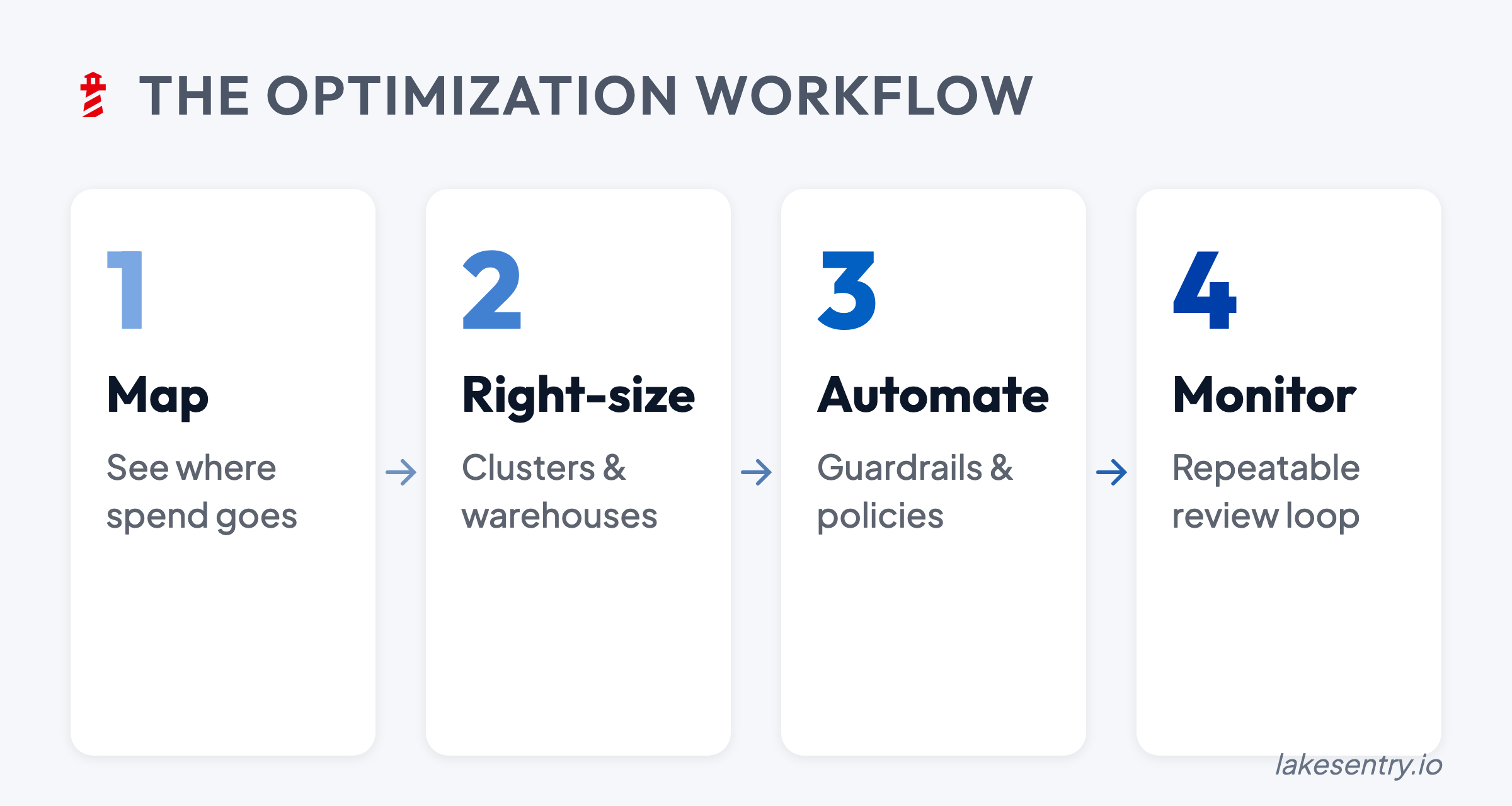
Databricks cost optimization starts with seeing where spend comes from: mapping cost to the workloads, teams, and clusters that drive it, then right-sizing compute and tuning warehouses from that map. This guide covers the five steps platform teams use — map, right-size, tune, automate, and monitor.
The quarterly cost review lands, and someone asks: “Why did Databricks go up 40%?” The room goes quiet. Not because the team doesn’t care — because nobody has a single view that explains which workloads drove the increase.
That’s where most Databricks cost optimization conversations start: not with a plan, but with a mystery. And the instinct, understandably, is to start cutting.
The problem is that cutting without visibility usually trades one surprise for another. You right-size a cluster and break a downstream SLA. You shorten a warehouse timeout and slow down the BI team’s morning dashboards. You turn off a “dev” resource that turns out to be the only working staging environment.
The first step to optimizing Databricks cost isn’t cutting anything. It’s seeing what’s actually happening.
What Makes Databricks Cost Hard to See
Databricks pricing runs on DBUs, which are abstract units that meter differently across compute types. A job on all-purpose compute burns DBUs at roughly 2-3x the rate of the same job on jobs compute. SQL warehouses have their own rate. Serverless bundles infrastructure into a higher DBU price. The same logical workload can cost $4 or $40 depending on where it runs.
Layer on top of that: most organizations run multiple workspaces, each with its own clusters, jobs, warehouses, and tagging practices. Cost data exists, but it’s usually missing the one thing you actually need: who owns the spend, and why it changed.
That’s the structural challenge: Databricks isn’t expensive in the abstract, but it’s complex enough that aggregate numbers don’t explain themselves, and the explanation is where the actual optimization lives.
Start with the Cost Map, Not the Scissors
The teams that reduce Databricks spend reliably have one thing in common: they know what they’re spending on before they start changing things. This sounds obvious. In practice, most environments skip straight to tuning without first establishing what’s actually driving cost.
A useful cost map answers three questions:
- By workload type: How much goes to jobs vs. SQL warehouses vs. interactive clusters vs. streaming? The split matters because the optimization levers are completely different for each.
- By team or project: Who is consuming what? Not just “which workspace” but which team, which pipeline, which business domain. Without this, every optimization conversation becomes a negotiation with no data.
- By time pattern: When does spend peak? Are there scheduling collisions? Is there a steady baseline of “always-on” compute that nobody’s watching?
Building this map from system tables is possible but labor-intensive. The bigger challenge isn’t the initial build — it’s maintaining it as teams reorg, pipelines get renamed, and new workspaces appear. The map has to stay alive, or it becomes another stale dashboard that nobody trusts. Once you have the map, the optimization priorities usually become obvious.
The hardest part of cost optimization is almost always figuring out where to look, not what to do once you’re looking.
Cluster Right-Sizing and Idle Detection
Interactive clusters are where the most avoidable spend hides, because they’re designed for convenience, not cost efficiency.
The pattern goes like this: someone spins up a cluster for notebook development. The instance type is generous because the work requires it at peak. The cluster runs all day. Peak usage is maybe 3 hours. The other 5 hours, it’s sitting idle, burning DBUs at the interactive rate, which is the most expensive rate Databricks offers.
Multiply that across a platform team of 15 people, each with their own interactive cluster, and you’re looking at significant spend that doesn’t correspond to any actual compute work. A cluster that runs 168 hours a week with 12 hours of actual task execution has a 7% utilization rate. Most batting averages are higher.
The fix isn’t to take clusters away, because interactive compute is legitimately important for development. The fix is structural:
- Auto-termination defaults. Every interactive cluster should have an auto-termination timeout. The default of “never” is the most expensive default in Databricks. 30-60 minutes covers most interactive workflows without being annoying.
- Cluster policies. Cap instance types and worker counts for interactive use. Developers rarely need 8-node clusters for notebook work. If they do, make it an explicit request with a justification.
- Separate interactive from production. Jobs that started as notebooks and got promoted to “scheduled” should move to jobs compute. The DBU rate difference alone is worth the migration effort.
For idle detection at scale, the diagnostic approach is straightforward: compare total cluster uptime against actual task execution time, per cluster, per week. Resources where the ratio is below 20% are candidates for review. (See the waste detection docs for how LakeSentry classifies these signals.)
SQL Warehouse Optimization
SQL warehouse cost is deceptive because it combines three variables that move independently: sizing, scaling behavior, and uptime.
Sizing. Warehouses come in T-shirt sizes (2X-Small through 4X-Large), and the cost scaling is roughly linear: a Medium costs ~4x a 2X-Small. Many warehouses are oversized for their actual query load because someone picked a size during setup and never revisited it. The diagnostic: check the warehouse’s peak concurrent queries against its capacity. If peak concurrency is 3 and the warehouse can handle 20, it’s oversized.
Serverless vs. classic. Serverless warehouses eliminate the cold-start problem and infrastructure management overhead. They also cost more per DBU. The tradeoff is simple in theory: serverless wins when utilization is bursty (lots of idle time between queries), classic wins when the warehouse runs consistently. In practice, most teams default to serverless because it’s easier — which is fine for development, but worth revisiting for production BI workloads that run on predictable schedules.
Auto-stop. This is the single highest-ROI setting in Databricks SQL and the one most often misconfigured. A warehouse with auto-stop set to “never” costs the same whether it’s running queries or sitting idle at 3 AM. Setting auto-stop to 10-15 minutes catches most idle periods without affecting users. Serverless warehouses restart in seconds, so there’s almost no reason not to set aggressive auto-stop.
Photon: When It Helps and When It Doesn’t
Photon is Databricks’ native vectorized engine. It runs supported operations faster, but at a higher DBU rate. The net cost impact depends on whether the speedup outweighs the rate increase.
Where Photon reliably saves money: large scans, heavy aggregations, filter-intensive queries, wide table reads. The wall-clock reduction more than offsets the higher per-DBU cost.
Where Photon doesn’t help: Python UDFs (Photon can’t accelerate them), small datasets where the speedup is negligible, ML training workloads, and anything dominated by I/O rather than compute. In these cases, you’re paying the higher rate without the corresponding speedup.
The mistake most teams make is enabling Photon globally because “faster is better.” That’s true for the workloads Photon accelerates. For everything else, it’s just a more expensive way to do the same work.
The practical approach: enable Photon selectively, starting with your heaviest SQL and ETL workloads. Compare total job cost (not just runtime) before and after. If total cost goes down, keep it. If it doesn’t, turn it off for that workload. The honest answer is sometimes “Photon doesn’t help here,” and that’s a useful finding since it removes a variable from your optimization equation.
Predictive Optimization and Unity Catalog
Databricks’ built-in predictive optimization automatically manages table maintenance operations: compaction, OPTIMIZE, VACUUM, file sizing. It’s genuinely useful for reducing storage costs and improving read performance on Delta tables that would otherwise accumulate small files over time.
What it doesn’t do: optimize compute cost. Predictive optimization works at the table level — it doesn’t know which jobs are expensive, which clusters are idle, or which teams are driving cost increases. It’s a storage and query performance feature, not a cost management feature.
This is a common source of confusion: teams enable predictive optimization expecting their Databricks bill to drop, then discover that compute is 80%+ of their spend, and compute optimization requires an entirely different set of levers.
Unity Catalog itself contributes to cost management indirectly, by providing a governance layer that makes it possible to track who accesses what. Governance creates the conditions for attribution, but someone (or something) still has to do the attribution work.
Performance Tuning That Saves Money
Some optimizations reduce runtime and cost simultaneously. These are worth prioritizing because they make workloads faster and cheaper.
Partition pruning. A query that scans an entire table because the partition filter doesn’t match the physical layout is doing 10-100x more I/O than necessary. The symptom: a query that “should be fast” takes minutes, and the Spark UI shows a full table scan. The fix is usually straightforward — align the query’s filter predicates with the table’s partition columns. When this works, the cost reduction can be dramatic.
Shuffle reduction. Joins and aggregations that produce large shuffles are the most common performance bottleneck in Spark. A poorly planned join can turn a 5-minute job into a 45-minute job. The 40 extra minutes are pure cost. Look at the Spark UI’s stage breakdown: stages with large shuffle writes and long task durations are the candidates.
Caching strategy. Disk caching and Delta caching reduce repeated reads from cloud storage. For workloads that re-read the same data (iterative ML, BI dashboards hitting the same tables), caching can cut I/O cost significantly. For single-pass ETL, caching adds overhead without benefit.
Runtime version. Clusters pinned to old Databricks runtimes miss engine improvements — better Adaptive Query Execution, improved Delta read paths, smarter shuffle handling. The workload keeps running, which is why nobody updates the runtime, but it runs slower than it would on a current version. Checking whether your heaviest workloads run on a current LTS runtime is a small effort with occasionally large payoff.
For a detailed walkthrough of the seven most common cost drivers and how to diagnose each one, see 7 reasons Databricks spend changes.
Automation: From Visibility to Action
After going through the manual optimization cycle a few times, most teams start asking: “Can we automate this?”
The answer is yes, but the sequence matters.
Automation works when it follows a trust ladder:
- See. Automated monitoring surfaces cost changes and their drivers. No action — just visibility, delivered consistently.
- Understand. Each flagged change comes with context: which workload, which owner, whether it’s expected. The team reviews and builds confidence in the signal quality.
- Approve. The system suggests actions — stop an idle warehouse, right-size a cluster, clean up an orphaned resource. A human reviews and approves each one, with an audit trail.
- Automate. Only for actions the team has approved repeatedly and trusts. Opt-in, bounded, reversible. With a kill switch.
The trap is when teams are jumping straight to step 4. Automation without explainability is a faster way to break things. A script that terminates “idle” clusters without knowing that one of them is a long-running streaming job is worse than no automation at all.
The principle is simple: automation shouldn’t outrun your understanding of what it’s automating. Start with consistent visibility. Let the decisions you’d make manually become obvious enough to codify them with guardrails.
An Optimization Workflow That Lasts
One-off optimization projects produce one-off results. The environment changes and costs drift back up. The pattern that actually works is a recurring weekly loop:
- Weekly review of the top cost movers, e.g. top 10.
- Ownership assignment. Every top mover gets an owner who can say “expected” or “needs investigation.”
- One change at a time. Treat cost changes like production changes. Small steps, measured impact, rollback path. The goal is to make steady, safe progress.
- Document and learn. Track what you changed, why, and what happened. Over time, this becomes a playbook that makes the next optimization faster.
The teams that sustain cost optimization are the ones with a consistent process — a weekly loop that catches drift before it compounds, and an ownership model that turns “someone should look at this” into “this particular person will look at it by Thursday.”
The most impactful Databricks cost optimization is having a normalized view of what’s happening across every workspace so the decisions about what to change become obvious before anyone has to guess. LakeSentry allows you to have a comprehensive view of your entire Databricks estate.
If you’re weighing tools for this, see the Databricks cost tools comparison.
See what's actually happening across your Databricks environment
Free tier — unlimited workspaces, no credit card. Connect in minutes.
Related reading
How Databricks pricing works: what a DBU is, list rates by compute type, plan tiers, cloud and region differences, and the costs the calculator misses.
When Databricks spend moves, start here. Seven common drivers from DBU multipliers to retry storms, with diagnostic steps and safe first moves for each.
Photon roughly doubles DBUs per hour. Whether it lowers your bill depends on the workload. Pricing math, what to enable, and how to measure on yours.
Evaluating Databricks cost tools? Compare them side by side →